
There are few moments in a country’s history that are more important than the adoption of a new constitution. If a constitution is implemented and upheld by the courts, then people are protected from their country’s most egregious abuses of power. The moment at which a constitution is adopted is important because these protections are often frozen in time and reflect the era in which they were adopted.
For instance, in 1215 the Magna Carta offered English citizens both timeless protections and safeguards that later became unimportant. On the one hand, the Magna Carta offered protections against illegal imprisonment which are now a hallmark of liberal democracies. On the other hand, the document also limited feudal payments to the crown which, thankfully, is a solution to yesteryear’s problems.
It is well known that the fall of the Berlin wall is the moment that marks the collapse of the Communist Bloc. Yet, a lesser-known impact of this change is that it prompted many countries formerly aligned with the Communist Bloc to draft new constitutions.
Data analysis offers a new and unique way to analyze laws and, on this occasion, the adoption of new constitutions. The technology allows us to analyze every constitution at the same time to find patterns about when they were adopted, what protections they offer, and – vitally – what is not protected. The tool that helps us do so is the R programming language.
The remainder of this blog post will be divided into three parts. Part 1 explains the notion of meta-data. Part 2 will introduce R code to investigate the constitutions meta-data which can be replicated by anyone with access to the dataset and R. Part 3 will discuss the results and highlight some important patterns that emerged.
What is Meta-Data?
Meta-data contains information about a document. For example, it tells us when a document was created, and the person who created it. In contrast to a document’s content, or its full text, meta-data contains readily analyzable information. As a result, the analysis of a corpus often starts with the analysis of its meta-data.
The constitutions corpus provides a good example of how to start an analysis with meta-data. We created the corpus in such a way that every filename of a constitutional text contains meta-data about that constitution such as which country the constitution belongs to and when the constitution was created, reinstated, or last revised. We can thus use the meta-data to track when the constitutions in our corpus were created.
Getting Started
The first step to any data analysis is setting up your working directory. You can learn to do so in Lesson 2 on the Data Science for Lawyers website. This lets R know what folder on the computer it will be interacting with. To verify what the computer is already interacting with, use the getwd() function. If you would like to change the working directory, you must assign a new working directory with the setwd() function.
getwd()
setwd("C:/Users/.../Legal Data/Constitutions")
Next, we need to load the data into R to commence the analysis of the meta-data. The following code shows you how to upload the data. Here, we are referring to a folder on our computer where the constitutions are stored and read them into R as text. You can learn more about data upload in Lesson 2.
##Load the text data from the folder in which they are stored into a dataframe
constitution_texts<-readtext("~/Legal Data/Constitutions")
Analysis of Meta-Data
Next, we will add a column to the dataset using the year the constitution was adopted. The decision to use the data in this way will have an impact on our results. This use assumes that the constitutions better reflect the values of the age in which they were adopted than those in the year they were last revised. We made this determination because revisions are often minor. It is important to remember that this assumption will have an impact on our results.
We draw on regular expressions introduced in Lesson 3 to extract information from meta-data. Regular expressions use patterns in text to find, extract or substitute textual information. Several strategies exist to craft regular expressions to mine meta-data. We may extract a specific pattern from a text string or “clean” an existing text string to eliminate information we do not need. In this post, we showcase both approaches. To get the year of adoption, we employ the latter strategy and clean our meta-data by reducing it to the information we want.
# Extracting the year of adoption
# We eliminate all non-numbers ("\\D+") from the meta-data string  and, since the year of adoption, is the first number, we then focus on the first four numbers.
constitution_texts$year_of_adoption <- as.numeric(substr(gsub("\\D+", "", constitution_texts$doc_id),1,4))
constitution_texts$year_of_adoption <-
as.numeric(constitution_texts$year_of_adoption)
Using the former strategy, we also want extract the name of the country from the filename to ensure that our data is presentable and easy to work with. We create a for-loop that goes through all filenames, splits them at the underscore plus digit and focuses on the first element of the ensuing list, which represents the country name. Note that we could have integrated the extraction of year of adoption into the same loop.
# Using a for loop to extract all country names.
# We start with an empty object of country names.
countryNames<-character()
# We then populate that empty object with country names, filename by filename.
for (name in constitution_texts$doc_id){
  countryName<-strsplit(name,"_\\d")[[1]][1]
  countryNames<-c(countryNames,countryName)
}
#storing the country name in a column of the data frame
constitution_texts$country <- countryNames
#ensuring that the results look reasonnable
constitution_texts$country
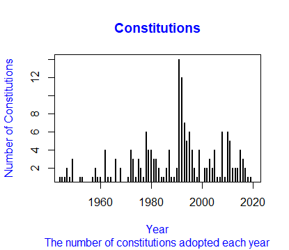
Then we graph the data. Since most countries adopted their constitutions since WWII this will serve as the starting point for the graph. The graph can easily be adjusted by changing the parameters set out in the code. Each line of code in the plot helps changes the default settings of the graph. Lesson 1 describes how to make these types of plots.
ConstiPerYear <- table(constitution_texts$year_of_adoption)
#A plot since 1945 which helps us see how many constitutions were #implemented each year since WWII
Since1945plot <- plot(ConstiPerYear,
                 type= "h", xlim=c(1945, 2020),
                 ylab= "Number of Constitutions",
                 xlab= "Year", main = "Constitutions",
                 sub= "The number of constitutions adopted each year",
                 col.lab="blue", col.main = "blue", col.sub = "blue",
                 lwd=2.5)
Finally, we create a table that outlines all the different countries that adopted new constitutions between 1990 and 1996. We do this by subsetting our meta-data (columns 3 and 4) based on the year in column 3 (year of adoption). The collapse of the communist bloc precipitated these adoptions.
#Create a data frama using only data from the 6 year period following the #spike in adoptions
YearnCountry <- subset(as.data.frame(constitution_texts[,3:4]),
                   constitution_texts$year_of_adoption >= 1990 &
                   constitution_texts$year_of_adoption <= 1996)
Finally, we turn this data into a .csv table and give it a name. This makes it easy to see the table in Excel. You can learn more about data export in Lesson 2.
#Write a CSV file to store the table
write.csv(YearnCountry, file = 'Adoption of Constitutions.csv')
Discussion: The Ripple Effect
The meta-data analysis offers several interesting insights into when and why constitutions were adopted.
There are a few moments in time when many constitutions were being adopted across the world. The moment when most constitutions were ratified occurred after the collapse of the Soviet Union in 1989.
In that year, the Berlin Wall fell, and few constitutions had recently been adopted. For instance, only one constitution was adopted in each of 1988 and 1989. This was followed by a spike in constitutional adoptions. 14 were adopted in 1991 and 12 were adopted in 1992.
This occurred, in part, because the Soviet Union dissolved into 15 new countries which all needed new constitutions after they abandoned communism. Yet, the collapse of the Soviet Union had a bigger impact than simply fragmenting one country. There were only 15 new countries that resulted from the collapse. Yet, 50 countries adopted new constitutions between 1990 and 1996.
Instead, the collapse had a more profound impact: It ended the global power struggle between capitalist and communist ideologies. This, in turn, precipitated constitutional reforms in the faraway lands of South America, Asia, and Africa. Countries around the world altered their governance and the protections they offered to their citizens in response to a definite end in the Cold War. The list of these countries, created above, is appended to the end of the post.
The impacts of the adoption of these new constitutions are that these countries codified the values that underpin their governance at the same time. As such, these constitutions should reflect the ideals of the 1990s. Some of these constitutions are thus likely to have codified ideals pertaining to gender equality, non-discrimination, political inclusion, and others. This being said, many modern concerns like the use of data, cyber-security, LGBTQ rights, or other recent issues are likely not codified. In the third post, we explore the changing content of constitutional protections over time.
After the fall of the Berlin Wall, the Cold War ended which caused a panoply of nations to adopt new constitutions. Like the Magna Carta, these constitutions will contain some concerns that are unique to its era, the 1990s, and some that will offer indispensable protections for generations to come. In determining which is which, your guess is as good as mine. What is clear, however, is that the fall of the Soviet Union was the event that precipitated these new beginnings.
| Year | Country | Years (cont) | Country (cont) |
| 1990 | Benin | 1992 | Togo |
| 1990 | Namibia | 1992 | Uzbekistan |
| 1991 | Bulgaria | 1992 | Viet Nam |
| 1991 | Burkina Faso | 1993 | Andorra |
| 1991 | Colombia | 1993 | Cambodia |
| 1991 | Croatia | 1993 | Czech Republic |
| 1991 | Equatorial Guinea | 1993 | Lesotho |
| 1991 | Gabon | 1993 | Peru |
| 1991 | Lao People’s Democratic Republic | 1993 | Russian Federation |
| 1991 | Macedonia Republic of | 1993 | Seychelles |
| 1991 | Mauritania | 1994 | Belarus |
| 1991 | Romania | 1994 | Ethiopia |
| 1991 | Sierra Leone | 1994 | Malawi |
| 1991 | Slovenia | 1994 | Moldova Republic of |
| 1991 | Yemen | 1994 | Tajikistan |
| 1991 | Zambia | 1995 | Armenia |
| 1992 | Djibouti | 1995 | Azerbaijan |
| 1992 | Estonia | 1995 | Bosnia and Herzegovina |
| 1992 | Ghana | 1995 | Georgia |
| 1992 | Lithuania | 1995 | Kazakhstan |
| 1992 | Mali | 1995 | Uganda |
| 1992 | Mongolia | 1996 | Gambia The |
| 1992 | Paraguay | 1996 | Oman |
| 1992 | Saudi Arabia | 1996 | South Africa |
| 1992 | Slovakia | 1996 | Ukraine |