Lesson 6

Preparing Metadata

To make sense of similarity patterns in legal documents, it is essential to start by extracting metadata. Meta data is the data that describes a document which often includes dates, sources and content.

For today's lesson, we will be working with Canadian labor agreements. Please download them and upload them into R.

# Load readtext package.

library(readtext)

# Load treaties into R.

folder <- "~/Google Drive/Teaching/Canada/Legal Data Science/Labor Agreements/EN/*"

# Upload the texts from that target folder.

treaty_texts <- readtext(folder)

# We start by creating two empty objects to which we will add the meta information.

treaty_partner <- character()
treaty_year <- numeric()

# We extract partner and year from each file name and then add it to the empty objects before proceeding to the next file name.

for (treaty_name in treaty_texts$doc_id) {

  treaty_name <- gsub(".txt|CDA-","",treaty_name)
  
partner <- strsplit(treaty_name, "_")[[1]][1]
treaty_partner <- c(treaty_partner,partner)  
year <- as.numeric(strsplit(treaty_name, "_")[[1]][2])

  treaty_year <- c(treaty_year,year)
}

treaty_texts <- cbind(treaty_texts,treaty_partner)
treaty_texts <- cbind(treaty_texts,treaty_year)

# Order by treaty year.

treaty_texts <- treaty_texts[order(treaty_texts$treaty_year),] 

Creating a Document-Term Matrix

We can now turn our treaty texts into data in order to prepare the similarity analysis. Similar to Lesson 5, we want to represent the texts as word frequency counts. This time, however, our focus is not on the terms but on the documents. So we create a Document-Term Matrix -- the simple inverse representation of a Term-Document Matrix.

We again start by creating a corpus object.

# Load package for text processing.

library(tm)

# We start by creating a corpus from the text.

corpus <- VCorpus(VectorSource(treaty_texts$text))

We then pre-process our treaty texts.

# Again, we get rid of variation that we don't consider conceptually meaningful.

corpus <- tm_map(corpus, removePunctuation)

corpus <- tm_map(corpus, content_transformer(tolower))

corpus <- tm_map(corpus, stripWhitespace)

corpus <- tm_map(corpus, removeNumbers)

corpus <- tm_map(corpus, removeWords, stopwords("english"))

We now want to use our corpus to create a Document-Term Matrix (DTM). In that matrix, every row is a document (here, a treaty) and every column is a term. The values are the frequencies of each term in a document. 

# Create a document term matrix.

dtm <- DocumentTermMatrix(corpus)

# For example, we restrict our analysis to all terms appearing in 2 or more documents.

dtm <- DocumentTermMatrix(corpus, control = list(bounds=list(global = c(2, Inf)))) 

# Finally, we transform the dtm from dataframe to numerical matrix.

dtm <- as.matrix(dtm)

Distance Measures I

When the textual similarity of documents is discussed, it is often done by refering to their "distance". The method intuits that similar documents will be "closer", and have a lesser distance, while for less similar documents will be "farther" and have a greater distance. Think of the word frequency counts of the DTM as the coordinates of each document in a vector space. Where these counts are identical, the two documents will occupy the same coordinates; if some counts differ, and others are the same, the two documents will be further apart, but not too distant; yet if the counts are very different and many terms exist in document A but not B, the coordinates of these two documents will be very far apart.

Statistical distance measures quantify this difference. They calculate how far apart two documents are based on their term frequency counts.

There are many different distance measures. We are now using a unigram representation of the texts. In that context, cosine similarity is often used to calculate the distance between documents. Here, however, we opt for a simpler binary distance measure that allows us to calculate the distance between documents by determining how many words, regardless of their frequency, are present in both documents. This distance measure is known as Jaccard distance. Jaccard distances have the useful advantage of being a measure between 0 (no distance, perfect similarity) and 1 (no similarity).  

We thus create a distance matrix using our DTM as input. 

# Create binary distance matrix checking whether or not a word appears in a document.

distance_matrix <- as.matrix(dist(dtm, method="binary"))

Distance Measures II

In law, context often matters, and as such a word frequency representation may not have enough detail to assess the similarity between documents. 

Instead, we can represent text through its constituent characters. The term "legal data", represented through its 5-character components, for example, would be "legal", "egal ", "gal d", "al da", "l dat" and " data". By calculating the Jaccard distance between these 5-character components, we can arrive at a more fine-grained comparison of text that takes word order into account. 

Note, however, that this is more computationally intensive. It will thus take considerably longer than calculating Jaccard distances between unigram representations of text. 

We use the package "stringdist" to compare the Jaccard similarity distances between treaties represented as 5-character components.

# Load packges

library(stringdist)

# Create a distance matrix

distance_matrix_5gram <- stringdistmatrix(treaty_texts$text,
treaty_texts$text,
method = "jaccard",
q = 5)

Visualizing Similarity Through Heatmaps

Heatmaps are a convenient way to visualize Jaccard distances. They color code high similarity (low distances) red and low similarity (large distances) yellow. We need two graphic packages to visualize the heatmap.

# Load packages.

library(ggplot2)

library(gplots)

heatmap.2(distance_matrix,

dendrogram='none',

Rowv=FALSE,

Colv=FALSE,

symm = TRUE,

trace='none',

density.info='none',

main = "Similarity labour treaties",

labCol = paste(treaty_texts$treaty_partner,treaty_texts$treaty_year,sep="-" ),

labRow = paste(treaty_texts$treaty_partner,treaty_texts$treaty_year,sep="-" ),

cexRow = 0.6,

cexCol = 0.6)

 ##

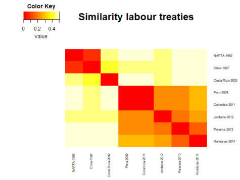
The heatmap is symmetrical, meaning that both axes display the same information and follow the same order. Here the heatmap is ordered chronologically from the earliest labor agreement (NAFTA 1992) to the latest (Honduras 2014). Based on the heatmap, we can identify three generations of Canadian labor agreements. The first is the NAFTA and Chilean treaty, which are both similar. The second one is made up Costa Rica agreement, which differs from all other agreements in our dataset. The third regroups all treaties signed since 2009.

Now we pass on to the more detailed heatmap of the labor treaties represented through their 5-character gram components. 

# no dendogram displayed. # column clustering. # row clustering. # heat map title.

heatmap.2(distance_matrix_5gram,
dendrogram='none', 

Rowv=FALSE, 

Colv=FALSE, 

symm = TRUE,

trace='none',

density.info='none',

main = "Similarity labour treaties", 

labCol = paste(treaty_texts$treaty_partner,treaty_texts$treaty_year,sep="-" ),

labRow = paste(treaty_texts$treaty_partner,treaty_texts$treaty_year,sep="-" ),

cexRow = 0.6,

cexCol = 0.6)

 ##

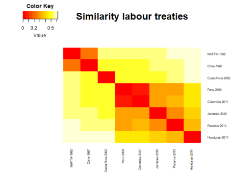
The overarching patterns are similar, but the results allow for a more refined comparison. The three generations still come out clearly, but we see an additional pattern which shows that the Peru and Colombia treaties are extremely similar - more so than any other agreement. In addition, the Honduras treaty, although similar to other agreements signed since 2009, appears more different than the prior heatmap suggested. This could indicate a movement towards a fourth generation of treaties.

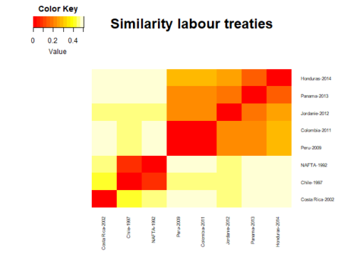
Importantly, our heatmaps have, up to now, been order based on the original dataframe. If we want to order our heatmap by similarity, we need to activate the hierarchical clustering built into the heatmap.2 algorithm. 

heatmap.2(distance_matrix,

dendrogram='none',

Rowv=TRUE,

Colv=TRUE,

symm = TRUE,

trace='none',

density.info='none',

main = "Similarity labour treaties",

labCol = paste(treaty_texts$treaty_partner,treaty_texts$treaty_year,sep="-" ),

labRow = paste(treaty_texts$treaty_partner,treaty_texts$treaty_year,sep="-" ),

cexRow = 0.6,

cexCol = 0.6)

 ##