Introduction
Networks are a powerful tool that help us better understand the law.
First, the law itself is full of networks: statutes that refer to each other, cases that cite prior cases, contracts that connect contractors, lawyers that work together and so forth. Network analysis helps understand the law’s network structures and this structure’s effects.
Second, network analysis comes with an entire toolkit to investigate network structures. Many of these measures have a foundation in human intuition. Consider the simple network below.
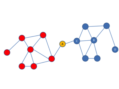
Ask yourself a couple of questions about this network.
- – Who is the most powerful actor in that network?
- – Who would you like to be friends with?
- – What new link is likely to be created next?
- – What is the likely social role of A or B?
- – What happens if A leaves the network?
- – What real life networks could this image represent?
Network analysis provides a framework to turn these intuitions into metrics. A node that has many connections, like node B, has a high “degree centrality” in the network. Node A, in contrast, has a high “betweenness” score, because it connects different groups of the same network.
Third, network analysis is scalable. That means it allows researchers to quickly analyze large amounts of information. What is the most important decision made by the Supreme Court of Canada in the last 20 years? A network analysis of citations by the Supreme Court of Canada’s judgements can provide an answer in seconds without manually reviewing thousands of cases.
Finally, network analysis provides an appealing way to visualize legal information.
What we will do in this lesson
We will primarily work on one aspect of legal network analysis: the citation networks of courts.
- 1. Using regexes to find citations
- 2. Creating a citation list
- 3. Finding most cited cases
- 4. Visualizing networks
- 5. Network measures
R Script
Using Regexes to Find Court Citations
Now, let's pick up where we left off in Lesson 3 and use regex to extract the citations from court decisions. Here, we will once again use Supreme Court of Canada data.# Activate package
library(readtext)
# Load the Supreme Court of Canada example data into a folder on your hard drive. Write the path to that target folder.
folder <- "~/Google Drive/Teaching/Canada/Legal Data Science/2019/Data/Supreme Court Cases/*"
# Upload the texts from that target folder.
scc <- readtext(folder)
pattern <- "\\[\\d+]\\s\\d+\\sS.C.R.\\s\\d+"
Creating a Citation List
We now want to extract instances where another Supreme Court decision is cited within our text. For that, we need to loop through all our texts and extract the citation.
As output, we want to have a dataframe with 2 columns. Column 1 will contain the case that contains the citation. Column 2 will contain the case that was cited.
Since we have multiple cases, we need to do a for-loop. We start with an empty shell that we will populate with citations.
# Here our dataframe has 2 columns for citing and cited cases.
all_citations <- data.frame(matrix(ncol = 2, nrow = 0))
Our loop will do two things. First, it will extract the cases that were cited. Second, we will add the case that had the citation in its text.
for (row in 1:nrow(scc)) {
# we first focus on the text of each decision
case_text <- scc[row, "text"] # we first focus on the text of each decision
# and search for our pattern in it
citation_matcher <- gregexpr("\\[\\d+]\\s\\d+\\sS.C.R.\\s\\d+", case_text)
# we then save all the cases cited in that decision
citations <- regmatches(case_text, citation_matcher)[[1]]
# second we focus on the name of the citing case
case_name <- scc[row, "doc_id"]
# and repeat so that every cited case can be accompanied by the name of the decision citing it
case_name <- strrep(case_name,length(citations))
case_name <- strsplit(case_name,".txt")[[1]]
# then we match cited and citing cases
citation_list <- cbind(case_name, citations)
# and save all these references in a dataframe
all_citations <- rbind(all_citations,citation_list)
}
Here, we see that a case will often cite another case multiple times. It is possible to incoporate this information into an analysis by using it to determine the weight of various network ties. Ties would be weighted more heavily when one case cites another multiple times.
Today, however, we want to simplify our data so that cases are connected by a tie irrespective of the number of times a citation occurs.
# We do that by eliminating duplicates.
all_citations <- unique(all_citations)
Finding Most Citing and Cited Cases
We can now use our citation list to find the most-citing and most-cited cases. To accomplish this, we use the function table(). This function provides us with frequencies of the values in our dataframe. We also sort our dataframe to make it easier to identify the most cited or citing case.
We start with the most-citing of our 25 cases.
# Based on our citation list, we can find the most citing and most cited cases in our list.
most_citing <- as.data.frame(sort((table(all_citations$case_name)), decreasing = TRUE))
most_citing
 ##
                   Var1 Freq
1    [2013] 1 S.C.R. 61   53
2   [2013] 1 S.C.R. 623   42
3     [2015] 1 S.C.R. 3   37
4   [2015] 2 S.C.R. 398   35
5   [2013] 1 S.C.R. 467   31
6   [2015] 3 S.C.R. 511   31
7  [2013] 3 S.C.R. 1101   27
8   [2015] 1 S.C.R. 613   24
9   [2014] 2 S.C.R. 167   23
10  [2016] 1 S.C.R. 130   23
11 [2015] 3 S.C.R. 1089   22
12   [2016] 1 S.C.R. 99   20
13  [2013] 2 S.C.R. 227   19
14  [2015] 1 S.C.R. 161   17
15  [2014] 2 S.C.R. 256   15
16     [2014] 1 SCR 704   12
17  [2016] 1 S.C.R. 180   11
18 [2017] 1 S.C.R. 1069   11
19  [2016] 2 S.C.R. 720   10
20  [2014] 2 S.C.R. 447    9
21  [2015] 2 S.C.R. 548    9
22 [2017] 1 S.C.R. 1099    9
23 [2013] 3 S.C.R. 1053    6
24  [2014] 1 S.C.R. 575    5
25    [2016] 2 S.C.R. 3    3
Hence, the most citing case in our network is Quebec (Attorney General) v. A, 2013 SCC 5, [2013] 1 S.C.R. 61.
We can do the same thing with the most-cited cases. This list will be considerably longer, so we restrict ourselves to the 50 most cited cases.
most_cited <- as.data.frame(sort((table(all_citations$citations)), decreasing = TRUE))
most_cited[1:50]
 ##
                    Var1 Freq
1    [1985] 1 S.C.R. 295    8
2    [2004] 3 S.C.R. 511    8
3    [1986] 1 S.C.R. 103    6
4    [2009] 2 S.C.R. 567    5
5    [1995] 3 S.C.R. 199    5
6   [1990] 1 S.C.R. 1075    5
7   [1997] 3 S.C.R. 1010    5
8    [2008] 2 S.C.R. 483    4
9    [1996] 2 S.C.R. 507    4
10   [2005] 3 S.C.R. 388    4
11   [2010] 3 S.C.R. 103    4
12   [2013] 1 S.C.R. 623    4
13    [1998] 1 S.C.R. 27    4
14  [2013] 3 S.C.R. 1101    4
15   [2012] 1 S.C.R. 433    4
16   [2014] 2 S.C.R. 257    4
17   [1986] 2 S.C.R. 713    3
18   [2011] 1 S.C.R. 396    3
19   [2012] 3 S.C.R. 555    3
20   [1999] 2 S.C.R. 203    3
21   [2000] 2 S.C.R. 307    3
22   [2005] 3 S.C.R. 458    3
23    [2013] 1 S.C.R. 61    3
24   [1984] 2 S.C.R. 335    3
25   [1998] 2 S.C.R. 217    3
26   [2002] 2 S.C.R. 235    3
27   [2003] 2 S.C.R. 236    3
28   [2004] 3 S.C.R. 550    3
29   [2003] 3 S.C.R. 571    3
30    [2010] 1 S.C.R. 44    3
31   [2011] 3 S.C.R. 134    3
32   [1984] 2 S.C.R. 145    3
33   [1999] 1 S.C.R. 688    3
34   [2010] 2 S.C.R. 650    3
35   [2004] 3 S.C.R. 698    3
36   [1989] 1 S.C.R. 927    2
37   [1990] 3 S.C.R. 697    2
38   [1995] 2 S.C.R. 513    2
39   [1996] 1 S.C.R. 825    2
40   [2004] 2 S.C.R. 551    2
41   [2006] 1 S.C.R. 256    2
42   [2007] 2 S.C.R. 610    2
43   [2008] 1 S.C.R. 190    2
44   [2011] 1 S.C.R. 160    2
45   [2011] 3 S.C.R. 471    2
46   [2011] 3 S.C.R. 654    2
47   [2013] 1 S.C.R. 467    2
48    [1988] 1 S.C.R. 30    2
49  [1989] 1 S.C.R. 1296    2
50   [1989] 1 S.C.R. 143    2
Hence, the most cited case in our network is R v Big M Drug Mart Ltd., [1985] 1 S.C.R. 295 and Haida Nation v British Columbia, [2004] 3 S.C.R. 511. The former is landmark Charter case and the latter is a leading case on the Crown's duty to consult Aboriginal groups.
Since we worked with a small sample of 25 decisions for this analysis, we should not make too much of these findings. If a similar analysis were applied to all Canadian Supreme Court cases, we would fine meaningful patterns about what cases are the most-cited and most-citing.
Visualizing Networks
We can next proceed to visiualizing this network in R.
A couple of packages in R deal with network analysis . The most popular of them is igraph.
library(igraph)
# The input is our 2-column matrix with the citation list.
citation_network <- graph_from_edgelist(as.matrix(all_citations), directed = TRUE)
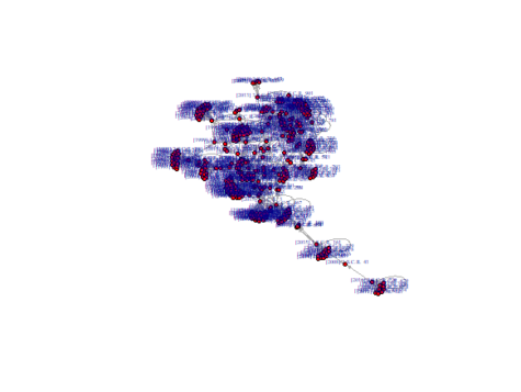
We can then use the plot() function to visualize the network.
plot(citation_network, layout=layout_with_fr, vertex.size=4,

vertex.label.dist=0.5, vertex.color="red", edge.arrow.size=0.2, vertex.label.cex=0.4)
##
While igraph is highly customizable, I personally prefer to work with self-standing network visualization tools. One of them is called "visone". It can be downloaded free of charge online: http://visone.info.
Network Measures
The igraph package can also calculate network measures. Several network measures exist that correspond to different node characteristics. Here we want to focus on two of them that are particularly useful for legal citation analysis:- Authority scores measure the importance of a node in a network based on the inward ties it attracts. In a legal citation network, this indicate that the case is a particularly important precedent.
- Hub scores measure the importance of a node in a network based on the outward ties it sends. In a legal citation network, this would correspond to a decision that cites all relevant authorities.
authority_score_network <- authority_score(citation_network, scale = TRUE, weights = NULL, options = arpack_defaults)
citation_authority <- as.data.frame(sort(authority_score_network$vector, decreasing=TRUE))
head(most_cited)
## Var1 Freq
head(citation_authority)
## sort(authority_score_network$vector, decreasing = TRUE)
hub_score_network <- hub_score(citation_network, scale = TRUE, weights = NULL, options = arpack_defaults)
citation_hub <- as.data.frame(sort(hub_score_network$vector, decreasing=TRUE))
head(most_citing)
## Var1 Freq
head(citation_hub)
## sort(hub_score_network$vector, decreasing = TRUE)
Dataset
Sample of cases from the Canadian Supreme Court in txt format. [Download]