Introduction
We now turn to the first of several lessons that treat text as data.
Benefits and shortcomings of text-as-data analysis
Treating text as data has one important advantage: scalability. While it takes time to read through cases, contracts and treaties, text-as-data techniques allow lawyers to process a lot of legal material efficiently and effectively in seconds.
Unfortunately, any conversion from text to data comes at the cost of losing semantic information. The meaning of words is partially derived from their context and part of that semantic context is inevitably lost when text is treated as data. Two consequences flow from this.
First, reading text and treating text-as-data are not substitutes; they are complements. A text-as-data analysis provides a bird’s-eye-view of the law by processing lots of information, but does not provide a detailed understanding. Reading text, on the other hand, provides detail and interpretive context that text-as-data analysis cannot match, but it is also time-consuming and thus necessarily restricted to a comparatively small number of selected documents.
Second, all text-as-data methods work with imperfect representations of text. The utility of a text-as-data analysis should not be evaluated by how accurately it reflects the text, but rather by how useful its insights about the text are. As we will see, usefulness often does not require semantic perfection.
Matching text-as-data methods with specific tasks
Since text-as-data methods are evaluated based on their usefulness and not how accurately they represent semantic nuances, the selection of text-as-methods depends on the task at hand. In this lesson, we will primarily work with term-frequency representations of text: We count the number of times a word appears in a document. As we will see, this simple representation of text is surprisingly useful for many tasks, but not for all. Sometimes we are only interested in particular words; sometimes, the grammatical form or the semantic context of words are crucial. There are many ways to represent and work with text. Which method is best, depends on what exactly you want to do. We will cover a few different application in this and the next lesson to guide you.
What we will do in this lesson
We will represent text as word frequencies to visualize and analyze the content and sentiment of legal texts.
-
1. Creation of a Text Corpus and Text Pre-processing
-
2. Creating a Term-document Matrix
-
3. Visualizing Word Frequency
-
4. Working with Bigrams
-
5. Dictionary approach I: Term mapping
-
6. Dictionary approach II: Sentiment Analysis
Useful resources
Grimmer, Justin, and Brandon M. Stewart. “Text as Data: The Promise and Pitfalls of Automatic Content Analysis Methods for Political Texts.” Political Analysis, 2013.
R Script
Encoding
Before we start with with text as data, a quick word on ENCODING. R needs to know how data is encoded to understand it properly. Some (non-English) letters are not supported through all encodings. Mostly, we will work with the standard UTF-8 encoding, which works well for English. In fact, we will get rid of all characters that do not fit into UTF-8.scc$text <- iconv(scc$text, "ASCII", "UTF-8",sub='')
# When working with French texts, for instance, use the following encoding:
scc$text <- iconv(scc$text, from="UTF-8", to="LATIN1")
Creation of a Text Corpus and Text Pre-processing
In this lesson, we return to our Supreme Court of Canada data and convert the judgments' text into data. To do that we, download and activate the tm package (one of several R packages that allow turning text into data) and create a corpus object.
# Load package.
library(tm)
# Create a corpus from the text.
corpus <- VCorpus(VectorSource(scc$text))
We should then do some processing on our corpus. There is some variation in our text that, for most tasks, we are not interested in. For instance, if we are interested in understanding the content of our corpus, it will not matter for our analysis whether a word is capitalised or not.
At the same time, pre-processing text is not a value-neutral exercise and it may affect your results. You thus need to be mindful what you do.
There are two ways to think about pre-processing choices. First, you could run the same analysis with different pre-processing combinations to make sure that your results are robust and do not vary strongly due to your pre-processing decisions. Denny and Spirling provide some useful guidance on this. Second, you could approach pre-processing from a more theoretical perspective and justify your pre-processing choices on conceptual grounds: "is the variation in the text that I am interested in for this particular task meaningfully distorted by this pre-processing step?"
# Here, we focus on getting rid of variation that we don't consider conceptually meaningful for investigating content variation in our SCC texts.
# Removing punctuation.
corpus <- tm_map(corpus, removePunctuation)
# Lowercasing letters.
corpus <- tm_map(corpus, content_transformer(tolower))
# Eliminating trailing white space.
corpus <- tm_map(corpus, stripWhitespace)
# Removing numbers.
corpus <- tm_map(corpus, removeNumbers)
A more controversial aspect is the removal of stopwords. Stopwords include "and", "or", "over", "our" etc. Take a look.
stopwords("english")
 ##
  [1] "i"          "me"         "my"         "myself"     "we"         "our"        "ours"       "ourselves"
  [9] "you"        "your"       "yours"      "yourself"   "yourselves" "he"         "him"        "his"
 [17] "himself"    "she"        "her"        "hers"       "herself"    "it"         "its"        "itself"
 [25] "they"       "them"       "their"      "theirs"     "themselves" "what"       "which"      "who"
 [33] "whom"       "this"       "that"       "these"      "those"      "am"         "is"         "are"
 [41] "was"        "were"       "be"         "been"       "being"      "have"       "has"        "had"
 [49] "having"     "do"         "does"       "did"        "doing"      "would"      "should"     "could"
 [57] "ought"      "i'm"        "you're"     "he's"       "she's"      "it's"       "we're"      "they're"
 [65] "i've"       "you've"     "we've"      "they've"    "i'd"        "you'd"      "he'd"       "she'd"
 [73] "we'd"       "they'd"     "i'll"       "you'll"     "he'll"      "she'll"     "we'll"      "they'll"
 [81] "isn't"      "aren't"     "wasn't"     "weren't"    "hasn't"     "haven't"    "hadn't"     "doesn't"
 [89] "don't"      "didn't"     "won't"      "wouldn't"   "shan't"     "shouldn't"  "can't"      "cannot"
 [97] "couldn't"   "mustn't"    "let's"      "that's"     "who's"      "what's"     "here's"     "there's"
[105] "when's"     "where's"    "why's"      "how's"      "a"          "an"         "the"        "and"
[113] "but"        "if"         "or"         "because"    "as"         "until"      "while"      "of"
[121] "at"         "by"         "for"        "with"       "about"      "against"    "between"    "into"
[129] "through"    "during"     "before"     "after"      "above"      "below"      "to"         "from"
[137] "up"         "down"       "in"         "out"        "on"         "off"        "over"       "under"
[145] "again"      "further"    "then"       "once"       "here"       "there"      "when"       "where"
[153] "why"        "how"        "all"        "any"        "both"       "each"       "few"        "more"
[161] "most"       "other"      "some"       "such"       "no"         "nor"        "not"        "only"
[169] "own"        "same"       "so"         "than"       "too"        "very"
In some legal contexts these words can matter a lot. Further, some words that we as lawyers may consider to be "noise" or unwanted stop words such as purely stylistic legal latin like "inter alia" , are not included in that stopword count. Hence as part of the exercise for this lesson, you will need to create a legal stopword list. For now, though, we just eliminate stopwords.
corpus <- tm_map(corpus, removeWords, stopwords("english"))
One other common pre-preprocessing step, stemming, whereby words are reduced to their root or stem, is something that must be done cautiously when applied to legal texts. The reason for that is because, in a legal context, words with the same stems can have very different meanings. For example, some stemmers group the word "arbitrary" and "arbitrator" to the same "arbitr" stem. As a result, stemming risks eliminating information that is useful to lawyers.
Creating a Term-document Matrix
Now that we have a pre-processed corpus, we can represent our text as data. More precisely, we can display it as a term-document-matrix where each row is a term and each column is a document, i.e. one of our judgments.# Create a term-document matrix.
tdm <- TermDocumentMatrix(corpus)
tdm <- as.matrix(tdm)
# We can for example sort our matrix by the word frequency in our corpus.
frequent_words <- sort(rowSums(tdm), decreasing=TRUE)
# Here are our most frequent words.
head(frequent_words, 8)
##
Visualizing Word Frequency
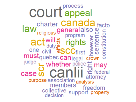
One of the advantages of R is that results are easy to visualize. For example, we can visualize how often a word is used through wordclouds. For that, we need to download and activate the wordcloud package.
# Load package.
library(wordcloud)
To make the wordcloud easily readable we reduce the information we want to display.
# It is easier to work with wordcloud if we tranform our file into a dataframe.
frequent_words <- as.data.frame(as.table(frequent_words))
colnames(frequent_words) <- c("word", "freq")
# In order not to overload the word cloud, we limit our analysis to the 50 most frequent words in the corpus.
most_frequent_words <- head(frequent_words,50)
Finally, we can proceed to the visualization.
# You can adjust the color to your liking.
wordcloud(most_frequent_words$word,most_frequent_words$freq, colors = brewer.pal(8, "Dark2"))
##
Working with Bigrams
Above we worked with single words -- unigrams. But we can do the same analysis with sequences of words -- ngrams. Here we use a sequence of 2 words -- bigrams.# This is our bigram function. R allows you to write your own functions. This is what we do here. We can then apply our function within the script similar to R's in-built functions.
bigrams <- function(x) unlist(lapply(ngrams(words(x), 2), paste, collapse = " "), use.names = FALSE)
# Creating a term-document matrix with bigrams.
tdm <- TermDocumentMatrix(corpus, control = list(tokenize = bigrams))
tdm <- as.matrix(tdm)
# Sort TDM find the 12 most frequent bigrams.
head(sort(rowSums(tdm), decreasing=TRUE), 12)
##
Dictionary Approach I: Term Mapping
Dictionary methods relate an outside list of terms to our corpus. This can be useful for a range of tasks. We may want to automatically check for the presence of absence of certain terms as part of a content analysis. Or we may want to select specific documents where specific signalling terms from our dictionary appear.
In this lesson, we use Dictionary methods for two tasks. First, we want to know whether appeals to the Supreme Court of Canada were successful or not. To do so, we will map signalling terms to automate this assignment. Second, we use a sentiment dictionary to determine whether the judges use a positive or a negative tone when in their judgements.
Here, we tackle the first of these tasks - classifying the outcome of decisions. For that, we can come up with two signalling terms that denote each outcome. Of course, rather than using one signalling term, we could use several.
# Load library
library(stringr)
success_formular <- "should be allowed"
reject_formular <- "should be dismissed"
We then check whether that word sequence is present and append it to our cases as success or reject.
success <- str_count(scc$text, success_formular)
reject <- str_count(scc$text, reject_formular)
Since each of these terms is potentially repeated, we substitute occurrences with "yes" and the absence of the term with "no".
success <- gsub("1|2","yes",success)
success <- gsub("0","no",success)
reject <- gsub("1|2","yes",reject)
reject <- gsub("0","no",reject)
Finally, we add the success and failure column to our dataset.
scc$success <- success
scc$failure <- failure
Take a look at the dataset using the View(scc) command. You will notice that some SCC cases are classified as both success and reject. How can that be? If you open the SCC judgment [2013] 1 S.C.R. 61.txt you will see that the Supreme Court allowed part of the appeal and dismissed another part. So our assignment of success and reject turned out to be correct. In general, it is prudent double check your results for accuracy.
Because legal texts often follow specific drafting rules and convention, such rule-based term mapping can work surprisingly well to map the contents of legal documents. But simple word mapping rules do not work for all tasks. Where no uniform signalling terms exist, researchers are better off to resort to more flexible machine-learning approaches that we will discuss in the section on Classification and Prediction.
Dictionary Approach II: Sentiment Analysis
Another dictionary approach uses outside word lists to investigate the sentiment of text. Essentially, that means that we count words with positive and negative connotation in a document to assess the sentiment or tonality of a document.
For example, political scientists have used sentiment analysis to investigate whether judges change their tone when dealing with particularly sensitive cases. We repeat a similar analysis here. The same approach, but with a different dictionary, could be used to look at other characteristics of legal texts, such as their prescriptivity, flexibility or use of legalese or outdated terms.
Let's start by downloading and activating the SentimentAnalysis package and by taking a look at its inbuilt sentiment dictionaries.
#Load package
library("SentimentAnalysis")
# The package comes with existing word lists of positive and negative words.
head(DictionaryGI$positive)
 ##
[1] "abide"     "ability"   "able"      "abound"    "absolve"   "absorbent"
head(DictionaryGI$negative)
 ##
[1] "abandon"     "abandonment" "abate"       "abdicate"    "abhor"       "abject"
Next, we want check how many of these positive and negative words exist in each text of our corpus. Do judges tend to use more positive or more negative language when framing their decisions.
# We count how many of positive and negative words exist in each text .
tdm <- TermDocumentMatrix(corpus)
text_sentiment <- analyzeSentiment(tdm)
When positive words outnumber negative ones, we classify a text as positive and vice versa. This is of course only an approximation but may nevertheless be helpful to group texts.
table(convertToBinaryResponse(text_sentiment)$SentimentGI)
 ## negative positive
       0           25
As it turns out, all judgments use more positive words than negative words.
Dataset
Sample of cases from the Canadian Supreme Court in txt format. [Download]
Exercises
1) Customizing your stop word list
You probably noticed that amongst the most frequent words are terms that tell us little about a decision’s content. For instance, it is unsurprising that “court” or “canlii” appears often. Take the list of most frequent words as a basis to create a legal stopword list.
1. Write your stopwords into the first column of a csv file. (Hint: Use the word frequency table to help you identify unwanted words)
2. Then upload the file and run your analysis again. What do you find?
# This sample code will help you.
stopwords <- read.csv("stopwords.csv", header = FALSE)
stopwords <- as.character(stopwords$V1)
stopwords <- c(stopwords, stopwords("english"))
corpus <- tm_map(corpus, removeWords, stopwords)
2) Expanding the sentiment analysis
1. Go back to the sentiment counts for each judgment. We saw that all decisions contain more positive words than negative ones. But do some contain more positive or negative words than others. Specifically, you may want to add your sentiment counts to the table with the success/failure classifications. Do decisions use more negative words when they dismiss an appeal?
2. What else, apart from sentiment, could you look for in these judgments? For instance, you may want to check how much latin legalese Canadian judges use. By adapting the sample code for stop words from above, you can create custom dictionaries to count the frequency of terms that you are interested in.